- 미래를 예측하거나, 과거를 복원하거나, 비어있는 데이터 갭을 채우거나, 이상치를 탐지하거나
- sound wave analysis
"Trend, Seasonality"
"Noise"
"auto-corelated time series - lag (이전 step에 의존적인)"
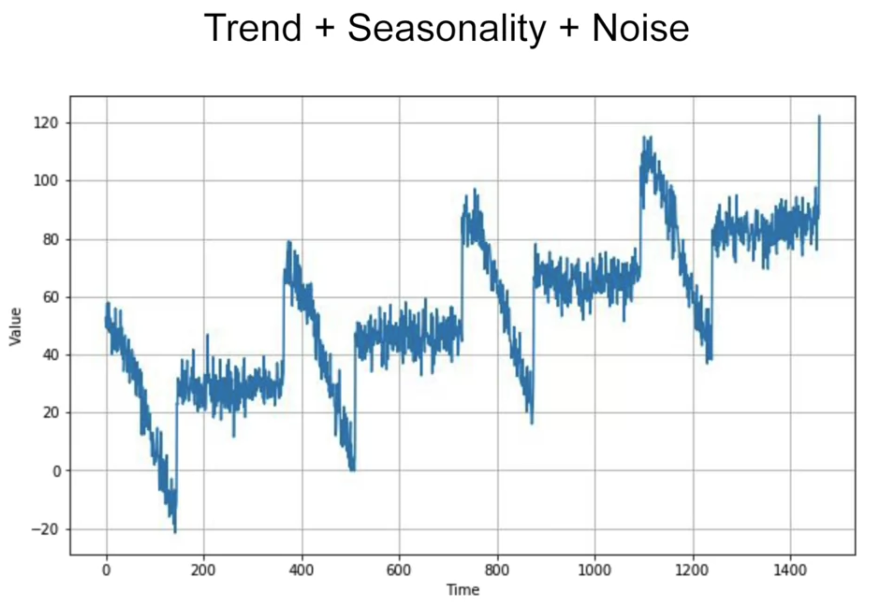
현실 데이터 : Trend + Seasonality + Autocorrelation + Noise
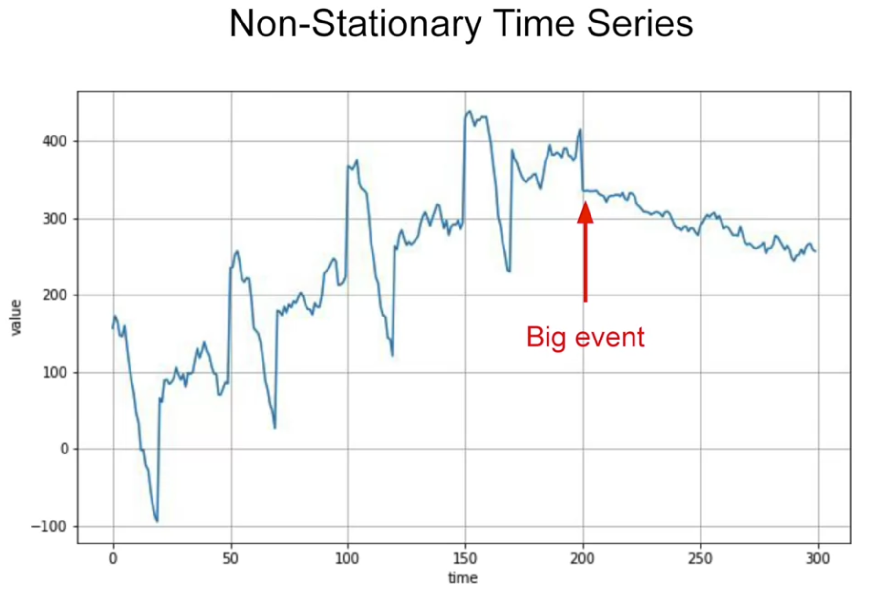
아래와 같은 "non-stationary time series" 도 있음
stationary --> 시간에 따라 behaviour가 바뀌지 않는다는 의미
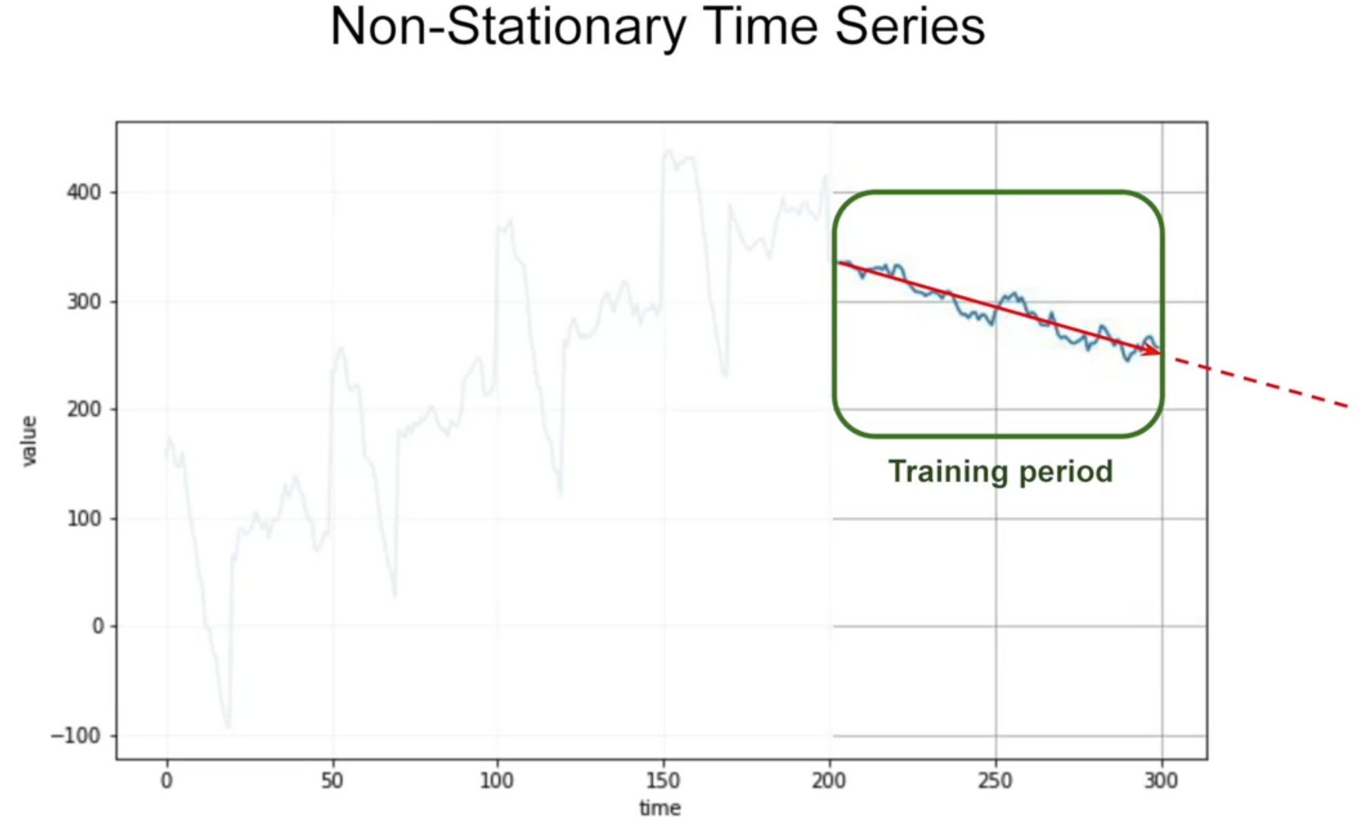
non-stationary --> optimal time window for training will vary
여기서 각종 time series 시뮬레이션 해볼 수 있음
위 데이터에서 일부를 확대하여 Naive Forecasting
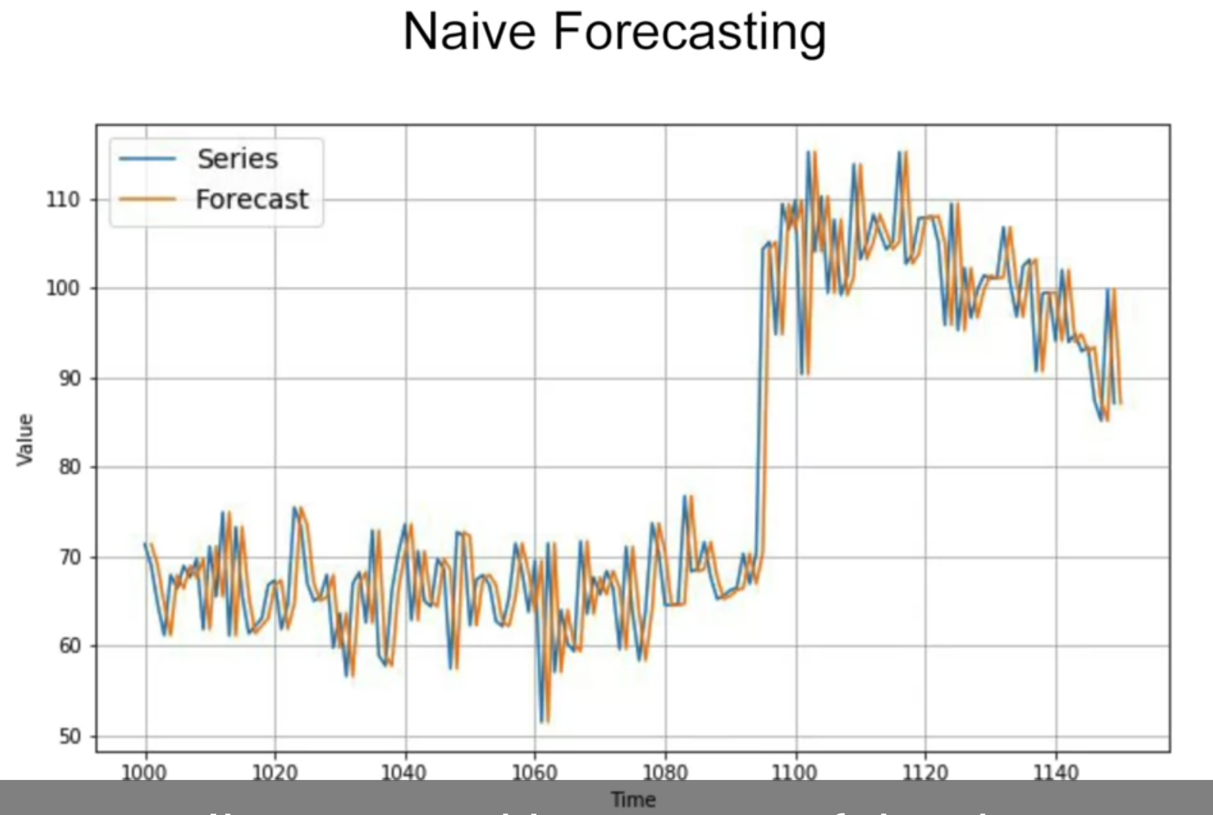
Naive Forecasting: 이전 값과 그 다음값이 동일할 것이라고 예측하는 것
how to measure performance? "Fixed Partitioning"
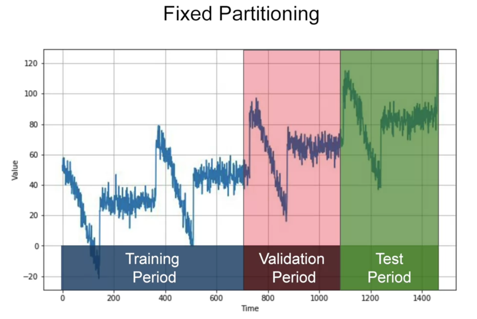
- 만약 데이터에 seasonality가 있다면, 각 period 에 모든 seasons가 있어야 할 것임 (일반적인 train-test split과는 다름)
- training period 가지고 학습, 그 다음 validation period도 포함해서 학습, 그 다음 test period도 포함해서 학습
---> test period가 현재 시점에서 가장 가까운 데이터이기 때문에 strongest signal in determining future values
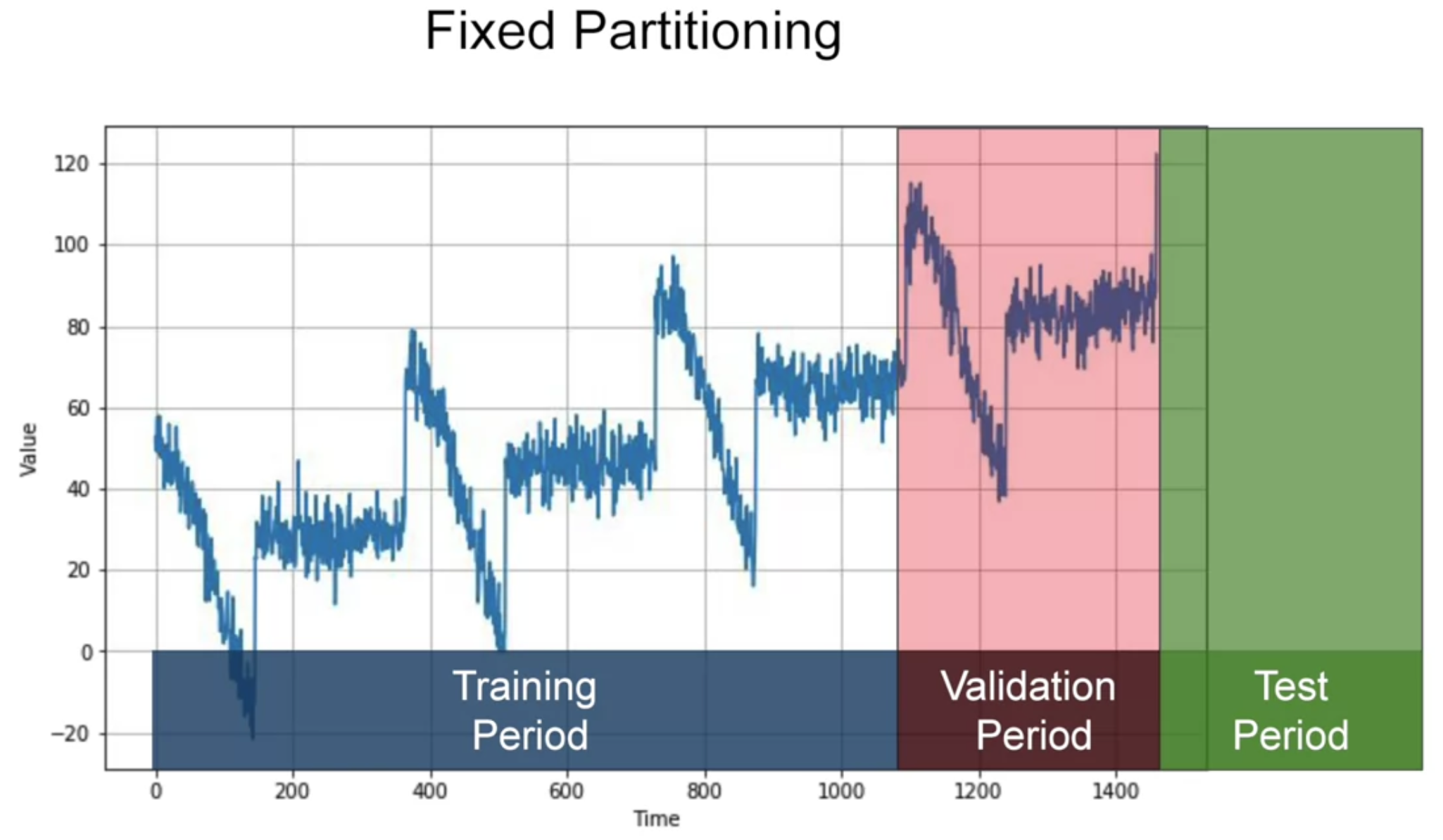
그래서 아래와 같이 할 수도 있다
또 다른 방법으로 "Roll-Forward Partitioning"
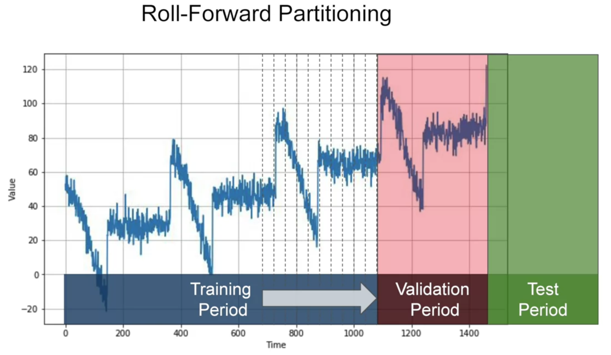
짧은 training period 로 시작해서 점점 늘려감 - fixed partitioning을 여러번 수행하는 것과 같음
[Metrics]
errors = forecasts - actual

mse = np.square(errors).mean()

rmse = np.sqrt(mse)

mae = np.abs(errors).mean()

mape = np.abs(errors / x_valid).mean()
If large errors are potentially dangerous and they cost you much more than smaller errors, then you may prefer the MSE. But if your gain or your loss is just proportional to the size of the error, then the MAE may be better.
tf.keras.metrics.mean_absolute_error(x_valid, naive_forcast).numpy()naive forcast의 MAE 를 baseline으로 잡고 시작
[moving average]
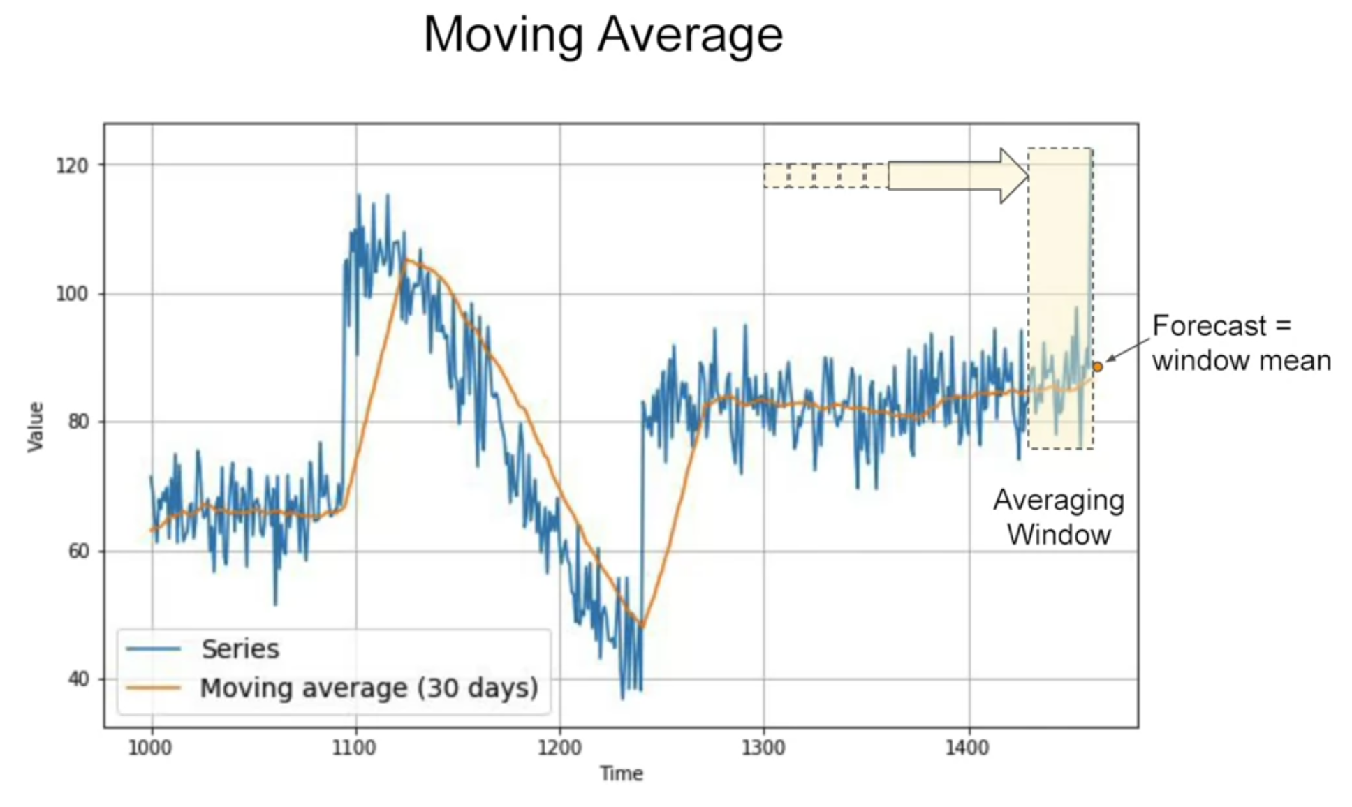
노란 구역 : averaging window 내 파란선의 average plot
-> noise를 일정 부분 제거해줄 수는 있으나, trend나 seasonality를 예측하는 것은 아님
[differencing] - trend와 seasonality 제거
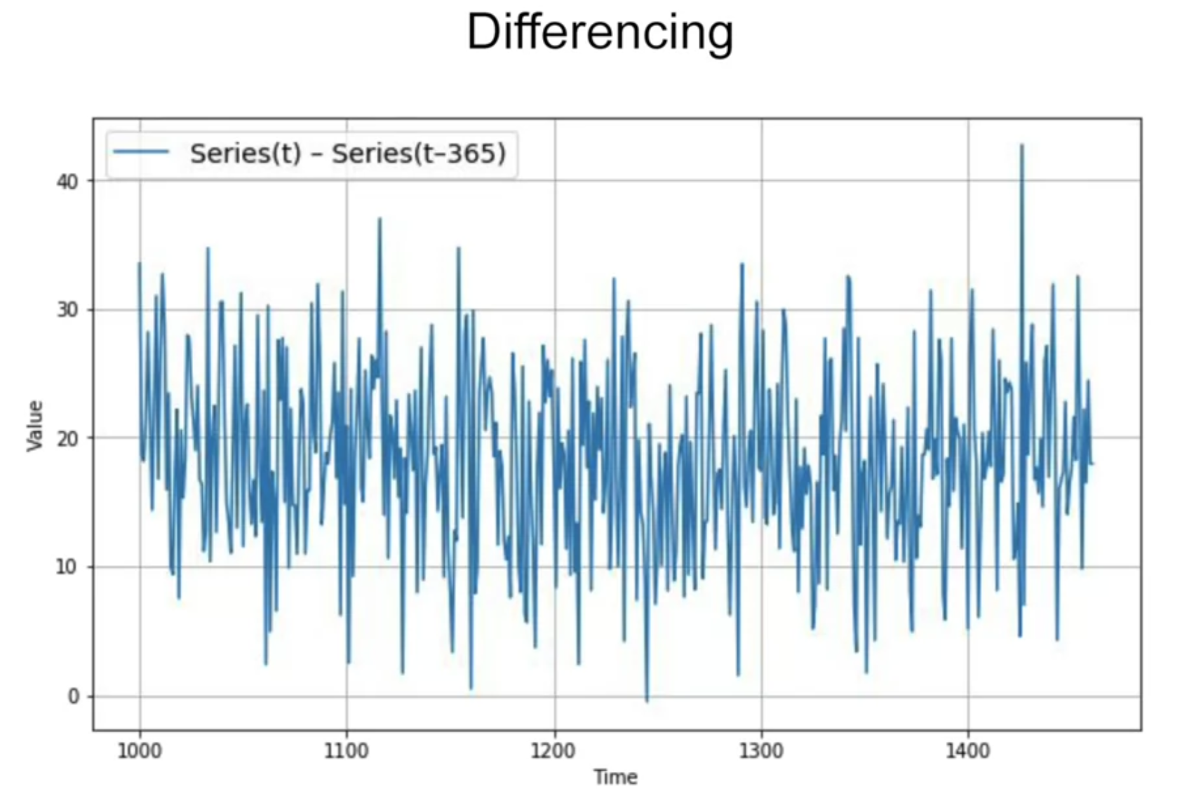
위 데이터의 경우 1년 전 데이터로부터 차이를 구함
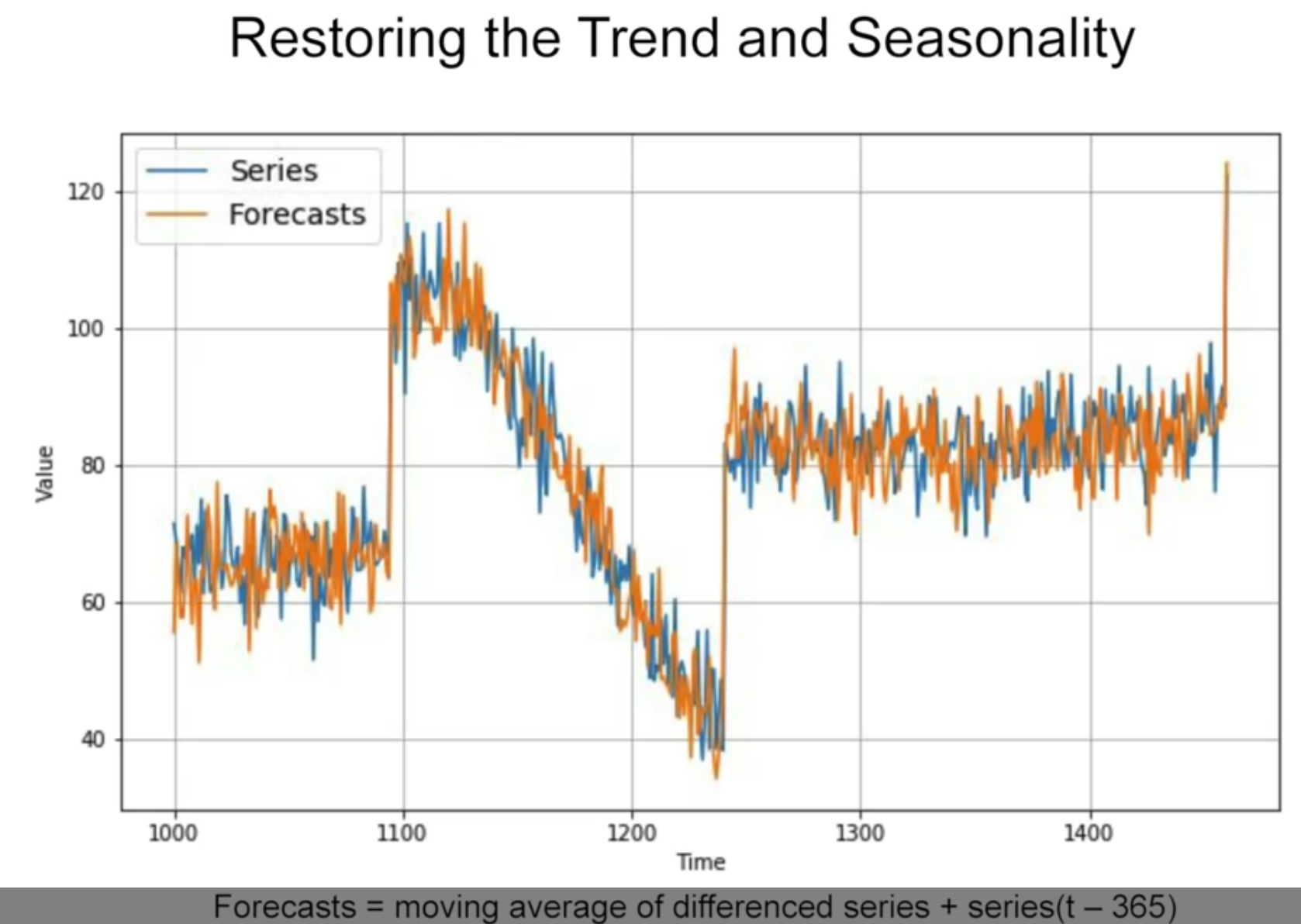
이 differencing time series에서 moving average를 구함 + 여기에 1년전 값을 더함
결과 : naive forcast보다 살짝 더 나음
더해진 1년전값에 노이즈가 있기 때문에 노이즈가 껴 있음 - 1년전 값에도 noise 제거를 한 후 실행하면
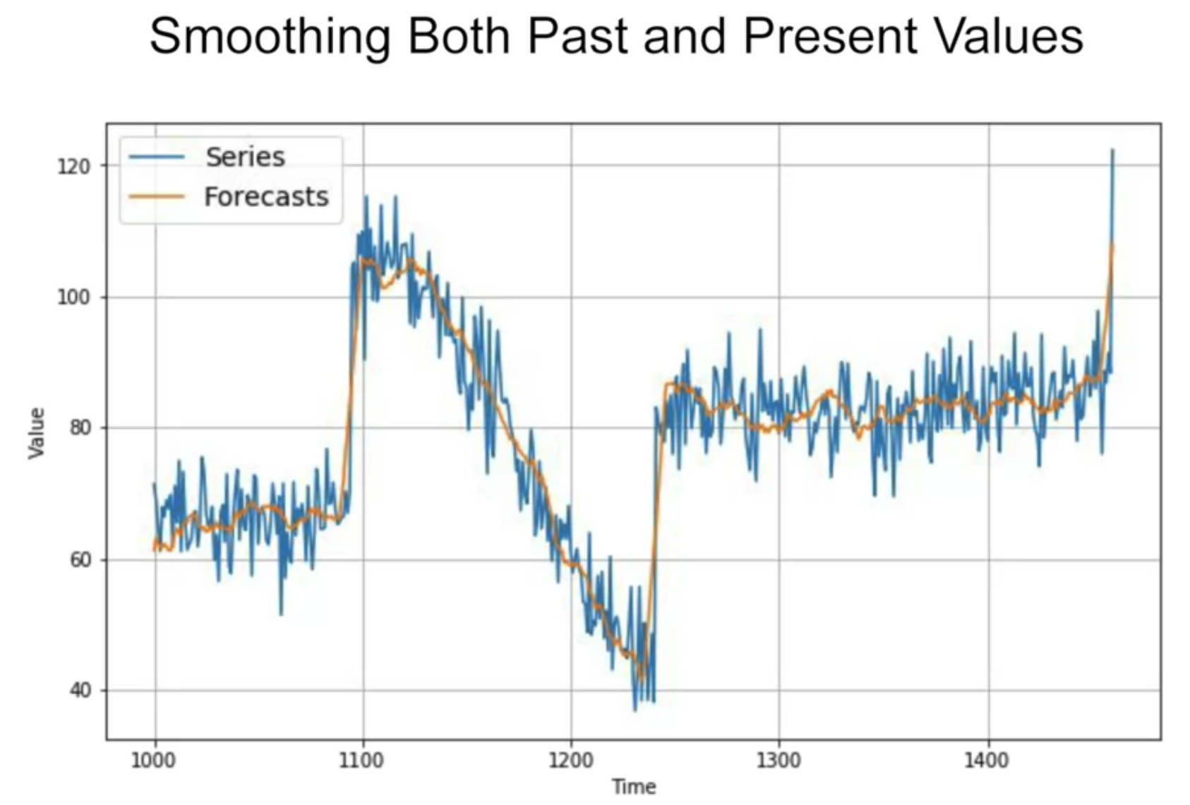
MAE 더 개선됨
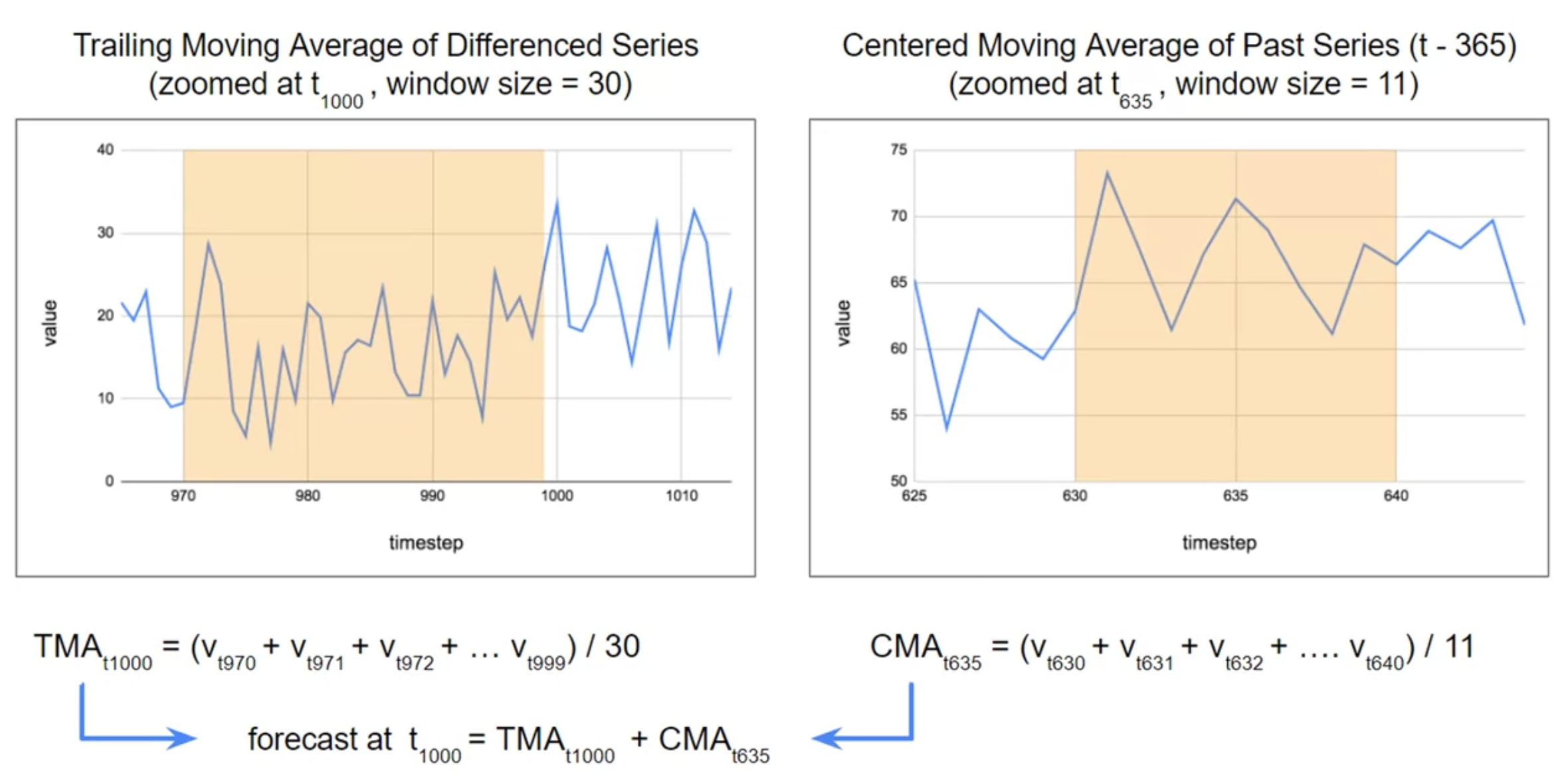
trailing moving average vs. centered moving average
현재의 값을 centered window 로 moving average를 구할 수는 없음 - 미래의 값을 모르기 때문에
대신에 과거의 값을 centered window로 구할 수는 있음
<시계열 데이터 합성한 후..>
train-valid split dataset
split_time = 1000

time_train = time[:split_time]
x_train = series[:split_time]

time_valid = time[split_time:]
x_valid = series[split_time:]
naive prediction (바로 이전값 복제하여 예측값으로 사용)
naive_forecast = series[split_time - 1 : -1]

keras.metrics.mean_squared_error(x_valid, naive_forecast).numpy())
keras.metrics.mean_absolute_error(x_valid, naive_forecast).numpy())
moving average --> smoothing effect
def moving_average_forecast(series, window_size):
	forecast = []

    for time in range(len(series) - window_size):
    	forecast.append(series[time:time + window_size].mean())

    forecast = np.array(forecast)

    return forecast

moving_avg = moving_average_forecast(series, 30)[split_time - 30:]

keras.metrics.mean_squared_error(x_valid, moving_avg).numpy())
keras.metrics.mean_absolute_error(x_valid, moving_avg).numpy())
differencing
해당 데이터에서 seasonality 가 1년으로 나오므로, t 값에서 (t-365) 값을 빼줄 것
diff_series = (series[365:] - series[:-365])
diff_time = time[365:]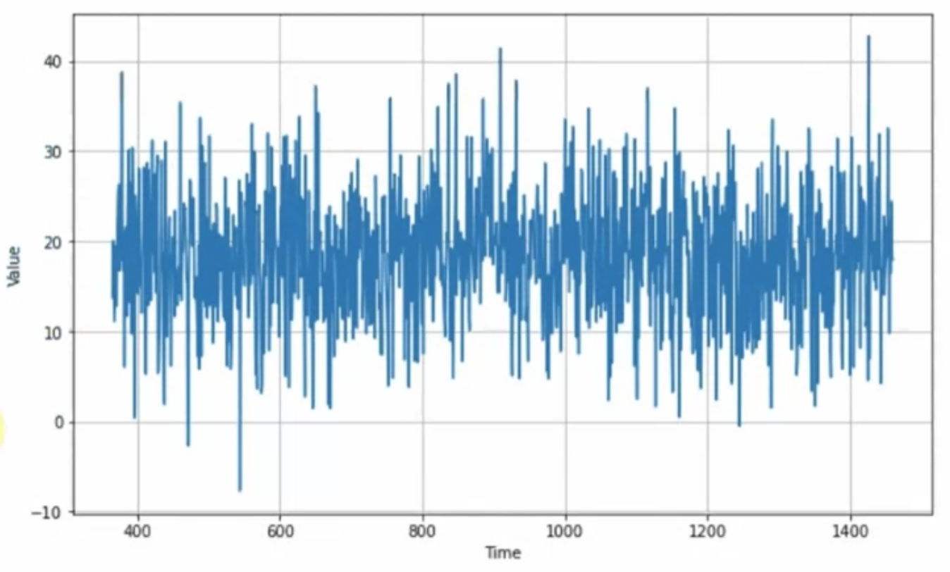
위 데이터에 moving average 적용
diff_moving_avg = moving_average_forecast(diff_series, 30)[split_time - 365 - 30 :]
diff_series = diff_series[split_time - 365:]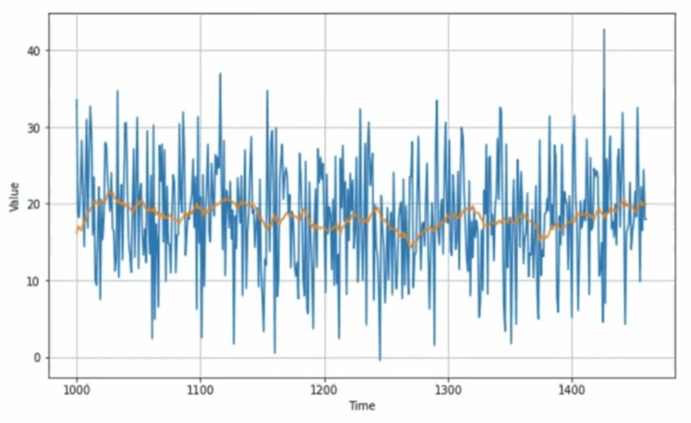
위에서 제외해주었던 (t-365) 값 다시 더하기
diff_moving_avg_plus_past = series[split_time - 365:-365] + diff_moving_avg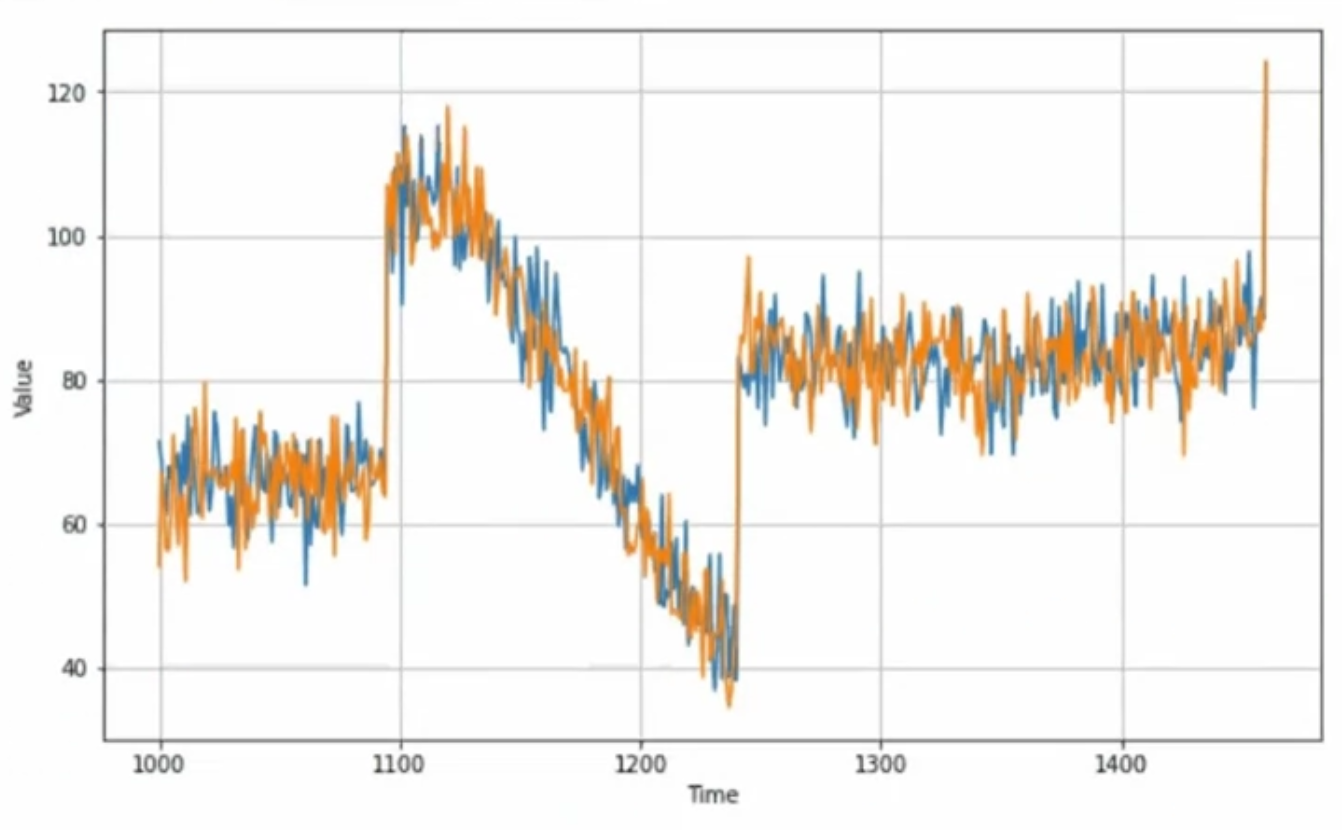
만약 (t-365) 값을 smoothing 해서 더한다면?
diff_moving_avg_plus_smooth_past = moving_average_forecast(series[split_time - 365:-365], 11) + diff_moving_avg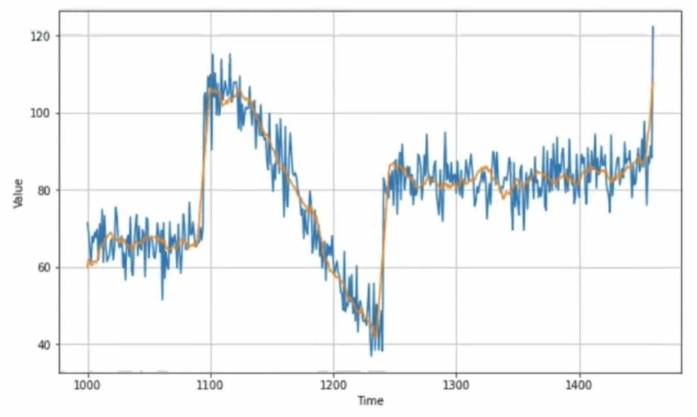
'인공지능 > tensorflow certificate' 카테고리의 다른 글
| 텐서플로우 자격증 시험을 위한 개발환경 구축 및 신청 (0) | 2022.08.23 |
|---|---|
| Sequences, Time Series, and Prediction(2) - Deep Learning (0) | 2022.08.22 |
| Natural Language Processing in TensorFlow(2) (0) | 2022.08.21 |
| Natural Language Processing in TensorFlow(1) (0) | 2022.08.21 |
| Convolutional Neural Networks in TensorFlow (0) | 2022.08.19 |